Code: Python3.7
Main packages: Pytorch, Captum, CUDA, Lime, Pillow
Read Time: ~ 15-30 min
Github: Explainability
What does Explainability mean:
Explainability does not just pertain to machine learning.
Explainability may be most prevalent in sociology. Someone comes up with a theory, and they set up a survey or a trial to test it; they see the results and repeat the process if needed. Physics, someone comes up with a theory, then find ways to test it ,i.e. God particle, quantum physics, etc. Just as a note, explainability doesn’t necessarily mean efficacy; the common drug acetaminophen is known to be unsure of why exactly its effects work. However, we can see that causality is a strong heuristic to look for in any domain for signs of explainability.
Explainability in STEM/life sciences/economics (rational man theory).
Rational man theory, or rational choice theory assumes that a person will always make prudent and logical decisions that yield the most benefits. As a side, bounded rationality suggests people frequently choose options without the ability to gather all pertinent information. Think of a weighted decision matrix. We are all frequently making decisions and weighing what is most important given x number of variables such as time and money. A decision is in large part based on the explainability of the model. Explainability being the extent to which we can no longer ask why. Explainability comes down to both the complexity of the problem as well as the circle of competence of the person making the decision. If we don’t understand why we are making decisions then we are far less likely to make quality decisions.
Data selection, feature engineering, transformations/permutations.
Data selection will be similar for the most part, assuming practitioners currently pay attention to the type of data and how well that data is understood. The added step of understanding business logic on data bias and risk assessment will assist the data selection process. Feature engineering will once again be very similar; following the first run of a model, an additional step will help this. That being understanding the business logic of the overall model/features/metrics and risk assessment. This includes looking at correlation, causation and creating semantic explanations for relevant behaviors. Once again all of this is dependent on model-specific methods vs model-agnostic methods. Model-specific will vary by model. Model-agnostic will vary by method.
Algorithm selection, hyperparameter tuning.
Explainability breaks down into model-specific explainability and model-agnostic explainability. Model-specific methods differ between each unique model; because of this it may be best to use model-agnostic methods. Model-agnostic methods will provide a general language to be able to work with a wider variety of models. Looking forward, this will also act as an easier framework to remember and to implement in personal projects, academics, jobs or the like.
Explainability is new; therefore, algorithms and frameworks are still being created and codified. Two popular model-agnostic methods are integrated gradients and shapley values. There are some limitations with these. When looking at what model to use, any model that uses gradient descent is differentiable therefore integrated gradients may be better. This will include neural networks, logistic regression, support vector machines, and the like. If the models are non-differentiable then shapley values will work. This will include trees, i.e. boosted trees and random forests.
Data science is a compound skill that draws from multiple disciplines. Intersection between programming, mathematics, and subject matter expertise.
One example of what a good mix of these attributes is a machine learning practitioner by the name of Marcos Lopez de Prado. He has deep domain expertise in investing, and has been able to apply machine learning, programming, and mathematics to help bring novel methods to the field. His domain experience allows him to be able to view the field of investing from an abstracted high level and detail oriented low level. The main thing that he brings to the table is his ability to understand why he is doing what he is doing. He has an idea of the overall market and that it’s really difficult to find alpha in regards to macro;therefore, leaving micro alpha to the playing field. He understands the type of data in the industry and where to get it, i.e. the data is most used is hardest to find novelty and the data that’s least used or least cleaned is the most valuable data.
What is the difference between interpretability and explainability.
Interpretability is the ability to see a models parameters and equations. Explainability is the ability to ask relevant why’s. When DARPA came out with their XAI challenge in 2016 they had 3 main goals: how to produce more explainable models, how to design the explanation interface, and how to understand requirements for effective explanations. So to understand explainability we can look empirically at how we learn. We might use counterfactuals, comparisons, context through stories, point out errors, or look for causality.
Contextualize the difference.
Let’s take an example of an image from autonomous driving. There are different conditions that the model has to account for. Imagine a freeze frame of a dangerous road. With an interpretable model the model will output red colored pixels signifying what areas of the image were used to predict that the road was dangerous. This could be a road with standing water. The model will highlight the areas with water signifying that it thinks that this is dangerous. With an explainable model, the reasons why the model are dangerous will be broken down more granularly. The model will show the pixels but it will also provide reasons for areas that are deemed safe versus dangerous. This could be that the model thinks the road is dangerous because there is standing water, there is rain, and there is a steep decline. The reasons why the model thinks the road is safe could be that it is day and that there are no other cars on the road. The goal is to know what areas are related to which predictions and the amount that the given predictions contribute to the overall prediction of the model. We then want to be able to codify this into higher level questions and answers.
Why does this impact data scientists, engineers, etc.
This impacts data scientists because it introduces a new way of looking at the problems that are being solved. Instead of focusing on maximizing or minimizing model metrics, explainability will focus on understanding that a is connected to b and the ‘why’ put into context.
This also impacts data scientists because it provides a new toolset to be able to provide understanding and efficiency in how machine learning is used. It impacts engineers because engineering is all about systems and causality, by adding explainability into the hands of variants of engineers, a lot of systems may become more ready for advancement.
As a slightly more abstracted idea, it may change the experiment before proofs mindset; instead of replacing math algorithms and proofs with testable math, i.e. running NN until your model learns what’s going on, we can start to move back to algorithms and proofs by looking at the why then by creating more articulate algorithms.
How will this affect workflow.
The processes that are added are done so in an attempt to limit, remove, or identify bias and to implement monitoring as well as implementing a design plan to add a human in the loop. First step is to get data and clean the data based on our working base of knowledge. The next step is the first added step which is to look at the business understanding on the data bias through risk assessment. Next define features, select a model and parameters, and define the scoring metrics along with calculating the accuracy. Once this is done, rinse and repeat as needed. The next added step is to do as we similarly did. Look at the business logic as well as the modelling, metric and feature understanding along with risk management. Persist the model and the code then predict using transformations and the trained model. The last added step is to look at the requirements for infrastructure required for monitoring, and to add process design plans to include human interactions in the loop. Overall it will add a lot more interaction in terms of key stakeholders as well as combining interaction with greater exploration of feature importance, accuracy and error.
Code pattern that demonstrates an interpretable model/practice versus an explainable one.
Interpretability in regards to deep learning, in one sense, may be broken down into 3 areas. General attribution, looks at the contribution of each input feature to the model output; layer attribution, looks at the contribution of each neuron in a given layer to the output; neuron attribution, looks at the contribution of each input feature on the activation of a particular hidden neuron.
# Pytorch with Facebook's Captum with an example of Integrated Gradients.
# Code from Pytorch tutorial with some changes.
!pip install captum

import numpy as np
import torch.nn as nn
import torch, torchvision
import torch.optim as optim
from torchvision import models
import torch.nn.functional as F
import torchvision.transforms as transforms
import torchvision.transforms.functional as TF
from captum.attr import IntegratedGradients
from captum.attr import visualization as viz

# install cuda: https://developer.nvidia.com/cuda-downloads
transform = transforms.Compose([transforms.ToTensor(), transforms.Normalize((0.5, 0.5, 0.5), (0.5, 0.5, 0.5))])
trainset = torchvision.datasets.CIFAR10(root='./data', train=True, download=True, transform=transform)
trainloader = torch.utils.data.DataLoader(trainset, batch_size=4, shuffle=True, num_workers=2)
testset = torchvision.datasets.CIFAR10(root='./data', train=False, download=True, transform=transform)
testloader = torch.utils.data.DataLoader(testset, batch_size=4, shuffle=False, num_workers=2)
classes = ('plane', 'car', 'bird', 'cat', 'deer', 'dog', 'frog', 'horse', 'ship', 'truck')

class Net(nn.Module):
    def __init__(self):
        super(Net, self).__init__()
        self.conv1 = nn.Conv2d(3, 6, 5)
        self.pool1 = nn.MaxPool2d(2, 2)
        self.pool2 = nn.MaxPool2d(2, 2)
        self.conv2 = nn.Conv2d(6, 16, 5)
        self.fc1 = nn.Linear(16 * 5 * 5, 120)
        self.fc2 = nn.Linear(120, 84)
        self.fc3 = nn.Linear(84, 10)
        self.relu1 = nn.ReLU()
        self.relu2 = nn.ReLU()
        self.relu3 = nn.ReLU()
        self.relu4 = nn.ReLU()

    def forward(self, x):
        x = self.pool1(self.relu1(self.conv1(x)))
        x = self.pool2(self.relu2(self.conv2(x)))
        x = x.view(-1, 16 * 5 * 5)
        x = self.relu3(self.fc1(x))
        x = self.relu4(self.fc2(x))
        x = self.fc3(x)
        return x

net = Net()
criterion = nn.CrossEntropyLoss()
optimizer = optim.SGD(net.parameters(), lr=0.001, momentum=0.9)

dataiter = iter(testloader)
images, labels = dataiter.next()
outputs = net(images)
_, predicted = torch.max(outputs, 1)

ind = 3
input = images[ind].unsqueeze(0)
input.requires_grad = True
net.eval()
Net( (conv1): Conv2d(3, 6, kernel_size=(5, 5), stride=(1, 1)) (pool1): MaxPool2d(kernel_size=2, stride=2, padding=0, dilation=1, ceil_mode=False) (pool2): MaxPool2d(kernel_size=2, stride=2, padding=0, dilation=1, ceil_mode=False) (conv2): Conv2d(6, 16, kernel_size=(5, 5), stride=(1, 1)) (fc1): Linear(in_features=400, out_features=120, bias=True) (fc2): Linear(in_features=120, out_features=84, bias=True) (fc3): Linear(in_features=84, out_features=10, bias=True) (relu1): ReLU() (relu2): ReLU() (relu3): ReLU() (relu4): ReLU() )
def attribute_image_features(algorithm, input, **kwargs):
    net.zero_grad()
    tensor_attributions = algorithm.attribute(input,target=labels[ind],**kwargs)
    return tensor_attributions

ig = IntegratedGradients(net)
attr_ig, delta = attribute_image_features(ig, input, baselines=input * 0, return_convergence_delta=True)
attr_ig = np.transpose(attr_ig.squeeze().cpu().detach().numpy(), (1, 2, 0))
print('Approximation delta: ', abs(delta)) # The lower the abs error the better the approximation.
Approximation delta: tensor([0.0001])
Delta is the difference between the total approximated and true integrated gradients. Using delta we can preview the underpinnings of the model and how the predicted and the actual compare to one another. We could preview a whole image as well with one output to one pixel. Although we can preview the error of each given pixel or feature it doesn’t necessarily provide us with insight into what exactly we’re looking at.
original_image = np.transpose((images[ind].cpu().detach().numpy()) + 0.5, (1, 2, 0))

_ = viz.visualize_image_attr(None, original_image, method="original_image", title="Original Image")
_ = viz.visualize_image_attr(attr_ig, original_image, method="blended_heat_map",sign="all", show_colorbar=True, title="Overlay of Integrated Gradients")

–
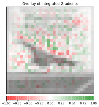
The image on the top is the original image of a ship. The image on the bottom is the overlay of gradient magnitudes showing what attributes contribute to the overall prediction of a ship. Integrated gradients are being used just as before. Although the image is really low resolution we can make out a set of pixels that were used for the prediction. By viewing certain pixels or superpixels we can see general behaviors of how the model is making predictions.
Explainability is a developing topic, especially when using images. A lot of scenarios that are being used involve having deep domain knowledge. This is where high level semantic feature explanations will come more into play, and are currently being worked on.
We do not want to tackle a complex problem with a complex solution
We have to take into account users limitations, i.e. if you have too many features, the user is not going to want to sit and digest all of it. One solution to this is to pick out a select few features and to view them individually aka locally. The other alternative is to use global importance measures by either averaging out a handful of selected features or by looking at all the features then taking the average.
Instead, we want to alter a workflow that is conducive to CACE and DRY principles to reduce redundant code patterns and offer explainability at all points of the data science process.
Both model-specific and model-agnostic methods act as a means for the DRY methodology. The typical machine learning workflow may consist of creating a basic model to test the application, increasing complexity, moving to a more complex mode.
Say you are trying to train a robot to pick up objects. You may start with a CNN to get a basic working model. Once you have a basic model you can quickly increase the complexity by adding layers, model parameters, then fine tune. After running the model a few times, you may move to a more complex model such as a Resnet-50 or the like then repeat the complexity and the fine tuning. If you use explainable methodologies, you can point to specific problem regions, and better understand the implications of any given model.
Highlight the difference between the blackbox model, and then show a model that has LIME wrapped on it, and demonstrates what features are relevant.
# !pip install lime
# Lime with ImageNet and Pytorch. Code pulled from 'github.com/marcotcr/', a lime library.

import numpy as np
import torchvision
import torch.nn as nn
import torch, os, json
import torch.nn.functional as F
import matplotlib.pyplot as plt
from PIL import Image
from torch.autograd import Variable
from torchvision import models, transforms
imagenet_data = torchvision.datasets.ImageFolder(root='/')
data_loader = torch.utils.data.DataLoader(imagenet_data, batch_size=4, shuffle=True)

# convert image to tensor and also apply whitening as used by pretrained model.
# Resize and take the center part of image to what our model expects.
def get_input_transform():
    normalize = transforms.Normalize(mean=[0.485, 0.456, 0.406], std=[0.229, 0.224, 0.225])
    transf = transforms.Compose([transforms.Resize((256, 256)), transforms.CenterCrop(224), transforms.ToTensor(), normalize])
    return transf

def get_input_tensors(img):
    transf = get_input_transform()
    return transf(img).unsqueeze(0) # unsqueeze converts single image to batch of 1

model = models.inception_v3(pretrained=True) # load ResNet50
# Load label texts for ImageNet predictions so we know what model is predicting
idx2label, cls2label, cls2idx = [], {}, {}
with open(os.path.abspath('imagenet_class_index.json'), 'r') as read_file:
    class_idx = json.load(read_file)
    idx2label = [class_idx[str(k)][1] for k in range(len(class_idx))]
    cls2label = {class_idx[str(k)][0]: class_idx[str(k)][1] for k in range(len(class_idx))}
    cls2idx = {class_idx[str(k)][0]: k for k in range(len(class_idx))}

def get_image(path):
    with open(os.path.abspath(path), 'rb') as f:
        with Image.open(f) as img:
            return img.convert('RGB')
img = get_image('dogs.png')
# Get prediction for image.
img_t = get_input_tensors(img)
model.eval()
logits = model(img_t)

# Predictions are logits; pass through softmax to get probabilities and class labels for top 5 predictions.
probs = F.softmax(logits, dim=1)
probs5 = probs.topk(5)
tuple((idx2label[c], p) for p, c in zip(probs5[0][0].detach().numpy(), probs5[1][0].detach().numpy()))
((‘Bernese_mountain_dog’, 0.93593), (‘EntleBucher’, 0.03844796), (‘Appenzeller’, 0.023756307), (‘Greater_Swiss_Mountain_dog’, 0.0018181851), (‘Gordon_setter’, 9.113298e-06))
Viewing the chosen model metrics is about as good as we can get in terms of interpretability with a neural network, and with using traditional out of the box models.
LIME:
from lime import lime_image
from skimage.segmentation import mark_boundaries
def get_pil_transform():
    transf = transforms.Compose([transforms.Resize((256, 256)),transforms.CenterCrop(224)])
    return transf

def get_preprocess_transform():
    normalize = transforms.Normalize(mean=[0.485, 0.456, 0.406], std=[0.229, 0.224, 0.225])
    transf = transforms.Compose([transforms.ToTensor(), normalize])
    return transf
pill_transf = get_pil_transform()
preprocess_transform = get_preprocess_transform()
def batch_predict(images):
    model.eval()
    batch = torch.stack(tuple(preprocess_transform(i) for i in images), dim=0)

    device = torch.device("cuda" if torch.cuda.is_available() else "cpu")
    model.to(device)
    batch = batch.to(device)

    logits = model(batch)
    probs = F.softmax(logits, dim=1)
    return probs.detach().cpu().numpy()
test_pred = batch_predict([pill_transf(img)])
test_pred.squeeze().argmax()

explainer = lime_image.LimeImageExplainer()
explanation = explainer.explain_instance(np.array(pill_transf(img)),
                                         batch_predict, # classification function
                                         top_labels=5,
                                         hide_color=0,
                                         num_samples=100000) # number of images that will be sent to classification functio
temp, mask = explanation.get_image_and_mask(explanation.top_labels[0], positive_only=True, num_features=5, hide_rest=True)
img_boundry1 = mark_boundaries(temp/255.0, mask)
plt.imshow(img_boundry1)
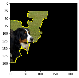
Above we can see the outline of our image showing how the image is selecting the edges. On top of this one may preview areas were attributed to being for and against the prediction.
Show how to do this yourself, so next time someone asks you what problem your code directly solves, you can tell (explain) them more than just the top-5 accuracy. - Above
Explainability as a workflow:
Explainability can be integrated into the workflow from the very beginning.
Explainability can be done in two ways; one is post-hoc explanations of a given training model, the second is to have an interpretable model. The interpretability is the ability to reveal all the mathematical operations and parameters in a system. We can then use interpretability to get the explainability. The process of adding in explainability from the beginning depends on the type of model.
We have simple models like linear regression and we have more complex models such as random forest regression or neural nets. With simple models we can look at all of the given features multiplied by their weights and then view the summation of these. This summation is additive which makes it more simple to understand. With more complex models it is harder to understand because we can’t single out simple individual equations. Instead we take all of the features that are going to our summation and we give them a credit. This method is applied to a number of models such as LIME, DeepLIFT, Shapley sampling, and more.
Resource constraints, data protection, downstream tasks are all affected by the inherent explainability of previous processes.
The number of people can have varying degrees of expertise. Resources may include available computational power, money, number of people, level of expertise. Explainability can be affected by any one of these. With more resources, the ability to understand a more complex problem is most likely to go up.
Data protection may be harder due to explainability potentially being heavily reliable on understanding what the values are and the business logic surrounding those values. There may be a need to tie the values to an individual, and most likely depends on a wide variety of contexts.
Why should we create explainable workflows?
Explainability in workflows helps improve or better define the following: debugging, stakeholder trust, insight in specific outputs, insight in high level concepts of models, and an overall understanding of how a model works. Let’s look further at the overall understanding. This can be further broken down into debugging, monitoring, transparency, and auditing. When looking at model performance, a common area of struggle is debugging, especially with more complex models such as random forests or neural nets.
By utilizing explainability we can see causes for why the model performs poorly on specific inputs. This naturally leads to better feature engineering and knowing why we are dropping certain features due to things such as redundancy. Let’s look at this in a little more detail. One way to look at this is that we want to be able to attribute a model’s prediction to its feature inputs. For example, we want to know why the prediction of hypoxemia (low oxygen in the blood) for an anesthetized patient is being predicted, not just that our model is predicting a 90% accuracy. Otherwise we aren’t sure which of the 7 different knobs the anesthesiologist needs to turn. We call this the attribution problem. One such attribution method is gradient based. This takes feature values * gradients ( xi * 𝜕y/𝜕x ). The gradient captures sensitivity of output with respect to the feature; remember partial derivatives for this.
Different thresholds for explainability; loan rejection and cancer diagnosis versus identifying a cat versus a dog.
Loan rejection: with a loan rejection we can use a model-agnostic method. This will most likely be represented as tabular data. With tabular data we can view feature importance relative to their impact on the models accuracy by graphing them as a barchart. We can ignore the features that have minimal or no impact on the models accuracy and focus on the alternative. Depending on what’s meant here for thresholds depends on the definition. If we are talking about model-specific methods then we can preview linear regression and feature importance levels. If we are talking about model-agnostic methods such as Shapley values we can use similar feature importances; however, with a slightly different meaning. In both cases the threshold would be both the overall accuracy of the model, as well as the individual feature importances and the degree to which those represent the overall accuracy.
Cancer diagnosis: an example of interpretability for cancer diagnosis could be the pixels being colored red or green as a representation of cancerous cells. This is not necessarily an explanation. Those are simply the models attributions of x connected to y outcome. What we are looking for is high level semantic explanations. We want the model to be able to say ‘I predict this is cancer because the bone density is 40% lower in this region compared to the overall average.’ We also want the model to provide us with semantic feature explanations for why it doesn’t think other areas are not cancerous like ‘This area was predicted 90% accuracy as not being cancerous based on the majority of healthy individual comparisons.’
Vertical, horizontal, and diagonal explainability. Vertical looks both up and down within a business unit, where explainability can be delivered to both managers and downstream users (upstream).
Explainability can be used to help users, both experts and laymen, to understand their model better. Explainability can also act as an extension to be able to gain better feedback loops from the end users. By letting a patient know what are the highest contributors to a prediction of a heart attack they can better work with their highest risk factors.
Horizontal explainability pertains to individuals across the same business unit (horizontal).
By better understanding what our model is doing we can better communicate with our co-workers. This can be in a corporate setting, an academic setting, or others. Horizontal communication will be altered by means of becoming more of a central focus. Metrics and interpretability will be important but focus will shift to being able to explain any given situation or result.
Diagonal explainability is a combination of vertical and horizontal explainability, where processes may be shared across business units, and explainability is desired for both end-users and principal agents (management). (downstream).
Diagonal explainability will have many of the benefits of horizontal with the possibility to have a greater impact. By providing explanations to at a diagonal level upper management can run a business with greater impact and employees can see more of why upper management is making certain decisions.
How will explainability practice empower data scientists?
Explainability will empower data scientists by providing them with a general language to be able to communicate why decisions are being made, or why bias is happening within a model. As mentioned before explainability will allow data scientists to be able to provide themselves and each other with high level semantic feature explanations. It will allow data scientists to be able to better explore their models and find what exactly is wrong with them. Remember that in a lot of models we have correlation which shows what the most important features that correlate with the outcome are. Some models also have causality. Explainability is being able to take correlation, causation, and other tools to enable higher level explanations.
DRY [don’t repeat yourself] and CACE [change anything change everything] can be alleviated if we have a deep understanding of our use-case, data, models, end-user, and subsequent downstream tasks.
Understanding the basic outline of our our libraries and models is a good place to start. By understanding the map we can more quickly know when and when not to use the map.
Below is a breakdown of popular libraries used for neural net interpretability and explainability; for Tensorflow and Pytorch. We can see below how each have broken down their models. By mixing this knowledge with other libraries and sources like academic papers, we can build a more robust and flexible view of explainability and how to implement it.
tf-explain:
- Activation Visualization: Visualize how a given input comes out of a specific activation layer.
- Vanilla Gradients: Visualize gradients on the inputs towards the decision.
- Gradients*Inputs: Variant of Vanilla Gradients weighting gradients with input values.
- Occlusion Sensitivity: Visualize how parts of the image affects neural network’s confidence by occluding parts iteratively.
- Grad CAM: Visualize how parts of the image affects neural network’s output by looking into the activation maps.
- SmoothGrad: Visualize stabilized gradients on the inputs towards the decision.
- Integrated Gradients: Visualize an average of the gradients along the construction of the input towards the decision.
Pytorch Captum:
General Attribution: input feature to the output of a model.
- Integrated Gradients
- Gradient SHAP
- DeepLIFT
- DeepLIFT SHAP
- Saliency
- Input X Gradient
- Guided Backpropagation
Guided GradCAM Layer Attribution: neuron in a given layer to the output of the model.
- Layer Conductance
- Internal Influence
- Layer Activation
- Layer Gradient X Activation
GradCAM Neuron Attribution: input feature on the activation of a particular hidden neuron.
- Neuron Conductance
- Neuron Gradient
- Neuron Integrated Gradients
- Neuron Guided Backpropagation
Noise Tunnel: computes any given attribution multiple times; adds Gaussin noise.
SmoothGrad: Mean of sample attributions. SmotthGrad Squared: Mean of squared sample attributions. Vargrad: Variance of sample attributions.
CODE: example of manually implemented, repetitive code (non pep-8 compliant) and poorly executed. Talk about how this relates to CACE and DRY, why, and offer solutions. Refer to solution as something that will be discussed in the future (incentivize continuous use of the course).
# DRY
#Use foor loops and functions when possible.
print(1)
print(2)
print(3)
# Utilize lists and for loops instead of repeat code.
nums = [1,2,3]
for x in nums:
    print(x)

# Decorators
# Decorators allow us to wrap a function with another function. i.e. func(func)
# Using decorators helps minimize redundancy and increases readability in code

# Wrong implementation using function w/ function
def SQUARED( x ):
    return lambda x:func( x )*func( x )

# pep-8 compliant
def squared(x):
    return lambda x: func(x) * func(x)

def x_plus_2(x):
    return x + 2

# Poorly implemented decorator
x_plus_2 = squared(x_plus_2)

# Better implementation of decorator
@squared
def x_plus_2(x):
    return x + 2

# Decorators with classes and use of classes themselves creates clean and efficient code.
# Classes are commonly used in both Pytorch and Tensorflow to create the initial neural network structure.
from random import randint
class Person(object):
    def __init__(self, name, turn):
        self.name = name
        self.turn = turn

    def get_name1():
        while 1:
            name = input("What is your name Player 1?")
            if name.isalpha() == False:
                print("\nPlease enter your name.\n")
            else:
                print("\nNice to meet you %s.\n" % name)
                return name
                break
    def get_name2():
        while 1:
            name = input("What is your name Player 2?")
            if name.isalpha() == False:
                print("\nPlease enter your name.\n")
            else:
                print("\nNice to meet you %s.\n" % name)
                return name
                break

Player1 = Person(Person.get_name1(), 1)
Player2 = Person(Person.get_name2(), 2)

print("Hello %s. You are Player 1." % Player1.name)
print("Hello %s. You are Player 2." % Player2.name)

# Class applied with decorator
 class Person(object):
    def __init__(self, name, turn):
        self.name = name
        self.turn = turn

    @classmethod
    def create(cls, turn):
        while True:
            name = input("What is your name Player 1?" % turn)
            if name.isalpha():
                break;
            print("\nPlease enter your name.\n")
        print("\nNice to meet you %s.\n" % name)
        return cls(name, turn)

Player1 = Person.create(1)
Player2 = Person.create(2)

print("Hello %s. You are Player 1." % Player1.name)
print("Hello %s. You are Player 2." % Player2.name)

# Include at beginning of pytorch code for reproducibility
# np.random.seed(1)
# torch.manual_seed(1)
# torch.cuda.manual_seed(1)