Code: Python3.7
Main packages: sklearn, pandas, xgboost, numpy
Read Time: ~ 15-30 min
Github: multi_Regression
Multiple Regression
Data Overview
Ames, Iowa: Alternative to the Boston Housing Data ( 2006 to 2010 )
- 2930 observations (Property Sales)
- Explanatory variables.
- 23 nominal - mainly dwelling structures.
- 23 ordinal - rate various items in property.
- 14 discrete - number of items; kitchens, bathrooms.
- 20 continuous - typically are dimensions.
NOTE: Remove houses > 4000 sqft.
We want to view housing data with different regression analyses.
# Import libraries
import numpy as np
import pandas as pd
import seaborn as sns
import xgboost as xgb
import lightgbm as lgb
import pandas_profiling
import matplotlib as lib
import matplotlib.pyplot as plt

from pydataset import data
from scipy.special import boxcox1p
from sklearn.pipeline import make_pipeline
from sklearn.kernel_ridge import KernelRidge
from sklearn.metrics import mean_squared_error
from sklearn.preprocessing import RobustScaler
from sklearn.preprocessing import LabelEncoder
from sklearn.model_selection import KFold, cross_val_score, train_test_split
from sklearn.ensemble import RandomForestRegressor,  GradientBoostingRegressor
from sklearn.linear_model import ElasticNet, Lasso,  BayesianRidge, LassoLarsIC
from sklearn.base import BaseEstimator, TransformerMixin, RegressorMixin, clone
# Import test and train set
test = pd.read_csv('Ames Housing Data/test.csv')
train = pd.read_csv('Ames Housing Data/train.csv')

# View shape of data
print('Shape of test set', test.shape)
print('Shape of train set', train.shape)
OUTPUT:
Shape of test set (1459, 80)
Shape of train set (1460, 81)
Exploratory Data Analysis
Housing price distribution.
lib.rcParams['figure.facecolor']= 'black'
lib.rcParams['axes.facecolor']= 'black'
lib.rcParams['lines.markersize'] = 10
lib.rcParams["scatter.marker"] = '.'
lib.rcParams['figure.titlesize']= 100
lib.rcParams['figure.figsize']=(18, 5)
plt.xticks(color='w')
plt.xlabel('Price', color='w')
plt.ylabel('Ratio', color='w')
plt.yticks(color='w')
plt.figtext(.5,.9,'Housing Price Distribution', fontsize=20, ha='center', color='w')

ax = sns.distplot(train.SalePrice, rug=True,
                  rug_kws={"color": "darkgrey", "lw": .3, "height":.1, 'alpha':1},
                  kde_kws={"color": "r", "lw": 1, "label": "KDE"},
                  hist_kws={"histtype": "step", "linewidth": 1, "alpha":1, "color": "r"})
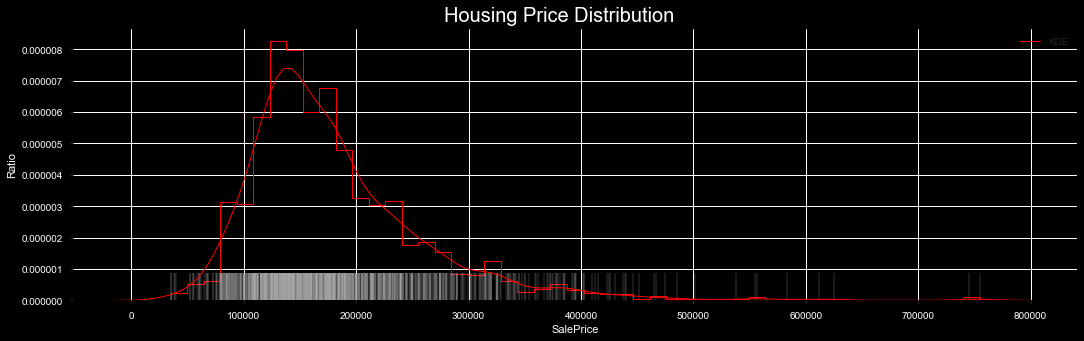
Skewness and Kurtosis
print("Skewness: ", train['SalePrice'].skew(), '| Biased towards the right due to a few high outliers.')
print("Kurtosis: ", train['SalePrice'].kurt(), '| Sharpness of peak, normal dist = 3')
print('Average House Price: ', round(train['SalePrice'].mean()))
OUTPUT:
Skewness:  1.8828757597682129 | Biased towards the right due to a few high outliers.
Kurtosis:  6.536281860064529 | Sharpness of peak, normal dist = 3
Average House Price:  180921.0
Review price to sqft to find outliers.
lib.rcParams['figure.facecolor']= 'black'
lib.rcParams['axes.facecolor']= 'black'
lib.rcParams['lines.markersize'] = 10
lib.rcParams["scatter.marker"] = '.'
lib.rcParams['figure.titlesize']= 100
lib.rcParams['figure.figsize']=(15, 10)
plt.xticks(color='w')
plt.xlabel('Price', color='w')
plt.ylabel('Squarefoot', color='w')
plt.yticks(color='w')

sns.scatterplot(data=train, x='SalePrice', y='GrLivArea')
plt.figtext(.5,.9,'Housing | Price Vs. Sqft', fontsize=20, ha='center', color='w')
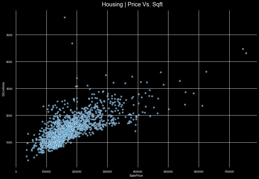
By removing the 4 outliers, we’re now able to bring our data closer to a normal distribution.
train = train[train['GrLivArea'] < 4000]
Skewness and Kurtosis - 2nd check.
print("Skewness: ", train['SalePrice'].skew(), '| Biased towards the right due to a few high outliers.')
print("Kurtosis: ", train['SalePrice'].kurt(), '| Sharpness of peak, normal dist = 3')
print('Average House Price: ', round(train['SalePrice'].mean()))
OUTPUT:
Skewness:  1.5659592925562151 | Biased towards the right due to a few high outliers.
Kurtosis:  3.8852828233316745 | Sharpness of peak, normal dist = 3
Average House Price:  180151.0
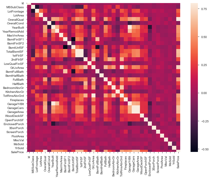
Correlations
#correlation matrix
lib.rcParams['figure.facecolor']= 'w'

corrmat = train.corr()
f, ax = plt.subplots(figsize=(12, 9))
sns.heatmap(corrmat, vmax=.8, square=True)
Positive correlation distribution
c = train.corr()
s = c.unstack()
positive_corr = s.sort_values(kind="quicksort", ascending=False)
negative_corr = s.sort_values(kind="quicksort")

positive_corr = positive_corr[positive_corr != 1]
negative_corr = negative_corr[negative_corr != 1]

lib.rcParams['figure.facecolor']= 'black'
lib.rcParams['axes.facecolor']= 'black'
lib.rcParams['lines.markersize'] = 10
lib.rcParams["scatter.marker"] = '.'
lib.rcParams['figure.titlesize']= 100
lib.rcParams['figure.figsize']=(24, 9)
plt.xticks(color='w')
plt.yticks(color='w')

plt.xlabel('Correlation', color='w')
plt.ylabel('Distribution', color='w')
sns.distplot(positive_corr)
plt.figtext(.5,.9,'Positive Correlation Distribution', fontsize=20, ha='center', color='w')

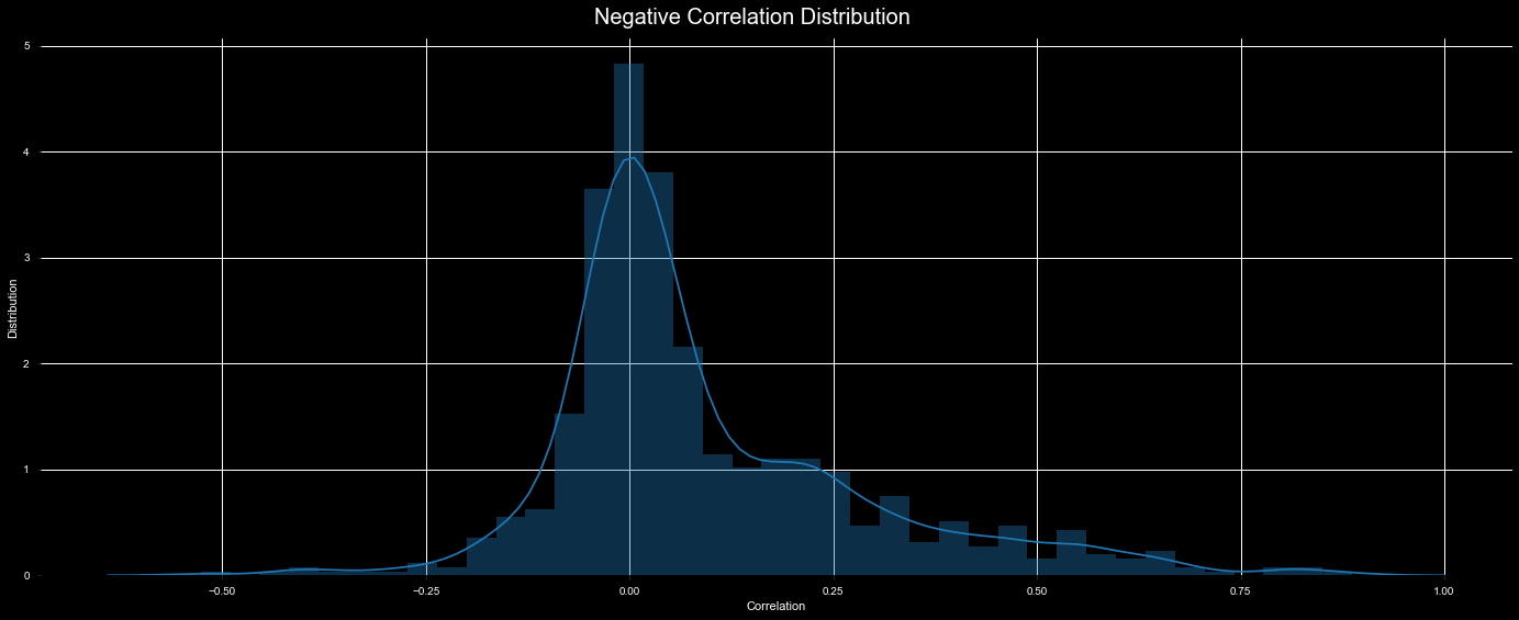
Negative correlation ditribution
lib.rcParams['figure.facecolor']= 'black'
lib.rcParams['axes.facecolor']= 'black'
lib.rcParams['lines.markersize'] = 10
lib.rcParams["scatter.marker"] = '.'
lib.rcParams['figure.titlesize']= 100
lib.rcParams['figure.figsize']=(24, 9)
plt.xticks(color='w')
plt.yticks(color='w')

plt.xlabel('Correlation', color='w')
plt.ylabel('Distribution', color='w')
sns.distplot(negative_corr)
plt.figtext(.5,.9,'Negative Correlation Distribution', fontsize=20, ha='center', color='w')
Clean, transform, and encode data.
cols = ('FireplaceQu', 'BsmtQual', 'BsmtCond', 'GarageQual', 'GarageCond',
        'ExterQual', 'ExterCond','HeatingQC', 'PoolQC', 'KitchenQual', 'BsmtFinType1',
        'BsmtFinType2', 'Functional', 'Fence', 'BsmtExposure', 'GarageFinish', 'LandSlope',
        'LotShape', 'PavedDrive', 'Street', 'Alley', 'CentralAir', 'MSSubClass', 'OverallCond',
        'YrSold', 'MoSold')

# Nans = no feature
feature_does_not_exist = [ 'BsmtQual', 'BsmtCond', 'BsmtExposure', 'BsmtFinType1', 'BsmtFinType2', 'FireplaceQu',
                           'GarageType', 'GarageYrBlt', 'GarageFinish', 'GarageFinish', 'GarageQual', 'GarageCond',
                           'PoolQC', 'Fence', 'MiscFeature' ]
Train
train.Alley = train.Alley.fillna("No access")

# Fill in select Nans
for x in feature_does_not_exist:
    train[x] = train[x].fillna('None')

train['Electrical'] = train['Electrical'].fillna(train['Electrical'].mode()[0])

# Turn into categorical information
train['MSSubClass'] = train['MSSubClass'].apply(str)
train['OverallCond'] = train['OverallCond'].astype(str)
train['YrSold'] = train['YrSold'].astype(str)
train['MoSold'] = train['MoSold'].astype(str)

# Labelencode
for x in cols:
    lbl = LabelEncoder()
    lbl.fit(list(pd.Series(train[x].values)))
    train[x] = lbl.transform(list(pd.Series(train[x].values)))
Skewness
numeric = train.dtypes[train.dtypes != "object"].index

# Check the skew of all numerical features
skewed_feats = train[numeric].apply(lambda x: pd.DataFrame.skew(x.dropna())).sort_values(ascending=False)
skewness = pd.DataFrame({'Skew' :skewed_feats})
skewness.head(10)
OUTPUT:br /> | Skew | | |:———–:|:———:| |MiscVal | 24.443364 | |PoolArea | 17.522613 | |LotArea | 12.587561 | |3SsnPorch | 10.289866 | |LowQualFinSF | 8.998564 | |LandSlope | 4.806279 | |KitchenAbvGr | 4.481366 | |BsmtFinSF2 | 4.248587 | |BsmtHalfBath | 4.128967 | |ScreenPorch | 4.115641 |
Fix Skewness
skewness = skewness[abs(skewness) > 0.75]
skewed_features = skewness.index
lam = 0.15
for feat in skewed_features:
    train[feat] = boxcox1p(train[feat], lam)
Get Dummies
train = pd.get_dummies(train)

train[train==np.inf]=np.nan
train.fillna(train.mean(), inplace=True)

X_train = train
y_train = train.SalePrice
Modelling
Kfold function randomizes our data, and splits it into train/test sets.
After kfold – run cross valiation. This runs our given model on the number of folds that we have specified.
This allows us to run a test on each section of our training data.
n_folds = 5

def rmsle_cv(model):
    kf = KFold(n_folds, shuffle=True, random_state=42).get_n_splits(train.values)
    rmse= np.sqrt(-cross_val_score(model, train.values, y_train, scoring="neg_mean_squared_error", cv = kf))
    return(rmse)
Lasso Regression
lasso = make_pipeline(RobustScaler(), Lasso(alpha =0.0005, random_state=1))
score = rmsle_cv(lasso)
print("\nLasso score: {:.4f} ({:.4f})\n".format(score.mean(), score.std()))
OUTPUT:
Lasso score: 0.0006 (0.0000)
Elastic Net
Linear regression with combined L1 and L2 as regularizer.
ENet = make_pipeline(RobustScaler(), ElasticNet(alpha=0.0005, l1_ratio=.9, random_state=3))
score = rmsle_cv(ENet)
print("ElasticNet score: {:.4f} ({:.4f})\n".format(score.mean(), score.std()))
OUTPUT:
ElasticNet score: 0.0008 (0.0000)
Kernel Ridge Score
KRR = KernelRidge(alpha=0.6, kernel='polynomial', degree=2, coef0=2.5)
score = rmsle_cv(KRR)
print("Kernel Ridge score: {:.4f} ({:.4f})\n".format(score.mean(), score.std()))
OUTPUT:
Kernel Ridge score: 0.0455 (0.0059)
Gradient Boost Regression
GBoost = GradientBoostingRegressor(n_estimators=3000, learning_rate=0.05,
                                   max_depth=4, max_features='sqrt',
                                   min_samples_leaf=15, min_samples_split=10,
                                   loss='huber', random_state=5)

score = rmsle_cv(GBoost)
print("Gradient Boosting score: {:.4f} ({:.4f})\n".format(score.mean(), score.std()))
OUTPUT:
Gradient Boosting score: 0.4439 (0.0246)
XG Boost Regression
model_xgb = xgb.XGBRegressor(colsample_bytree=0.4603, gamma=0.0468,
                             learning_rate=0.05, max_depth=3,
                             min_child_weight=1.7817, n_estimators=2200,
                             reg_alpha=0.4640, reg_lambda=0.8571,
                             subsample=0.5213, silent=1,
                             random_state=7, nthread = -1)

score = rmsle_cv(model_xgb)
print("Xgboost score: {:.4f} ({:.4f})\n".format(score.mean(), score.std()))
OUTPUT:
Xgboost score: 0.2112 (0.0250)
LGBM Regression
model_lgb = lgb.LGBMRegressor(objective='regression',num_leaves=5,
                              learning_rate=0.05, n_estimators=720,
                              max_bin = 55, bagging_fraction = 0.8,
                              bagging_freq = 5, feature_fraction = 0.2319,
                              feature_fraction_seed=9, bagging_seed=9,
                              min_data_in_leaf=6, min_sum_hessian_in_leaf = 11)

score = rmsle_cv(model_lgb)
print("LGBM score: {:.4f} ({:.4f})\n" .format(score.mean(), score.std()))
OUTPUT:
LGBM score: 0.3663 (0.0335)
Average of models
class AveragingModels(BaseEstimator, RegressorMixin, TransformerMixin):
    def __init__(self, models):
        self.models = models

    # we define clones of the original models to fit the data in
    def fit(self, X, y):
        self.models_ = [clone(x) for x in self.models]

        # Train cloned base models
        for model in self.models_:
            model.fit(X, y)
        return self

    #Now we do the predictions for cloned models and average them
    def predict(self, X):
        predictions = np.column_stack([
            model.predict(X) for model in self.models_
        ])
        return np.mean(predictions, axis=1)
Run class
averaged_models = AveragingModels(models = (ENet, GBoost, KRR, lasso))

score = rmsle_cv(averaged_models)
print(" Averaged base models score: {:.4f} ({:.4f})\n".format(score.mean(), score.std()))
OUTPUT:
Averaged base models score: 0.1140 (0.0061)