Code: Python3.7
Main packages: Pillow, Tensorflow, Protobuf, Tensorboard
Read Time: ~ 15-30 min
Github: cnn_tensorflow
CNN USPTO Analysis
Transfer Learning
Patents are filled with technical jargon and legal jargon. Typically, the information may be understood with enough time, or preexisting domain knowledge. Using machine learning and some creativity, I believe it’s possible to simplify this data for the average joe, like myself. Hopefully this project will turn into something that allows an individual to take their domain knowledge their idea and use a mix of a user interface and machine learning to find relavent patents and ideas on how a patent my be applicable to them.
To get Started:
- Follow the docs to install Tensorflow. Tensorflow Docs
- Download USPTO patent images. Select one tar file. The smalled size is ~ 6GB. USPTO Images
Convert images
USPTO images come in a tiff format. Tensorflow doesn’t support this so we need to convert it to another format such as JPG. After unzipping the USPTO images, the code below will run through all folders recursively and change any .tif to a .jpg. Run the code in the upper most directory.
import os
from PIL import Image # Pip install PIL
path = '//Tensorflow/workspace/patent_project/images/'
for root, dirs, files in os.walk(path, topdown=False):
    for name in files:
        print(os.path.join(root, name))
        if os.path.splitext(os.path.join(root, name))[1].lower() == ".tif":
            if os.path.isfile(os.path.splitext(os.path.join(root, name))[0] + ".jpg"):
                print("A jpg file already exists for %s" % name)
            # If a jpeg is *NOT* present, create one from the tiff.
            else:
                outfile = os.path.splitext(os.path.join(root, name))[0] + ".jpg"
                try:
                    im = Image.open(os.path.join(root, name))
                    print("Generating jpeg for %s" % name)
                    im.thumbnail(im.size)
                    im.save(outfile, "JPEG", quality=100)
                except Exception as e:
                    print(e)
Train/test split
Once we convert the files we can split the images into training and testing. Because the USPTO image set is so big, we can also take a smaller portion as a whole for our model. For the project I did a 70/30 split and used around 500 images total.
Annotate
Download the ‘labelImg’ desktop app. LabelImg annotates images by placing bounding boxes around the items that you want to identify.
NOTE: It’s helpful to look at the keyboard shortcuts for lableImg so you can annotate more quickly.
There are a handful of apps that assist with annotation, both video and images. For the most part, if a company really needs images to get annotated, they’ll hire it out as a mechanical turk job or to an agency that specializes in annotation.
LabelImg creates an XML file for each image, this is how the bounding box boundries for each image are created.
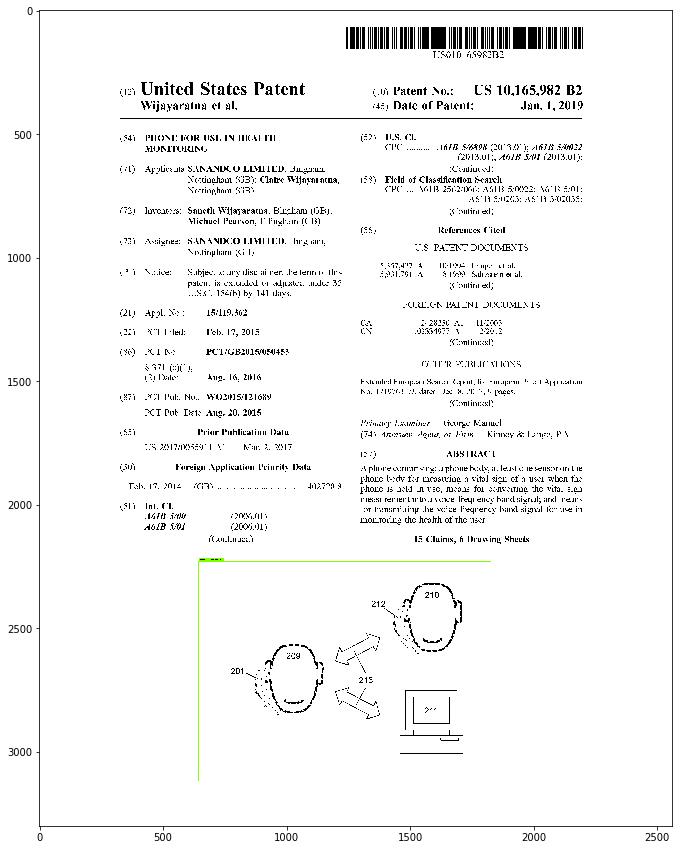
Example single annotation XML file:
<annotation>
    # Folder name
    <folder>1</folder>
    # Filename
    <filename>280.jpg</filename>
    # path to jpg image
    <path>/Volumes/LaCie/grant_yb2_20190101/2019-01/10/165/1/280.jpg</path>
    # Here's the size of our image. Width-Height-Depth
    <size>
        <width>2560</width>
        <height>3300</height>
        <depth>1</depth>
    </size>
    <object>
        # Annotation label
        <name>patent image</name>
        # Bounding box dimension - x:829,y:2235(bottom left corner) | x:1698,y:3104(top right corner)
        <bndbox>
            <xmin>829</xmin>
            <ymin>2235</ymin>
            <xmax>1698</xmax>
            <ymax>3104</ymax>
        </bndbox>
    </object>
</annotation>
Multiple Annotations
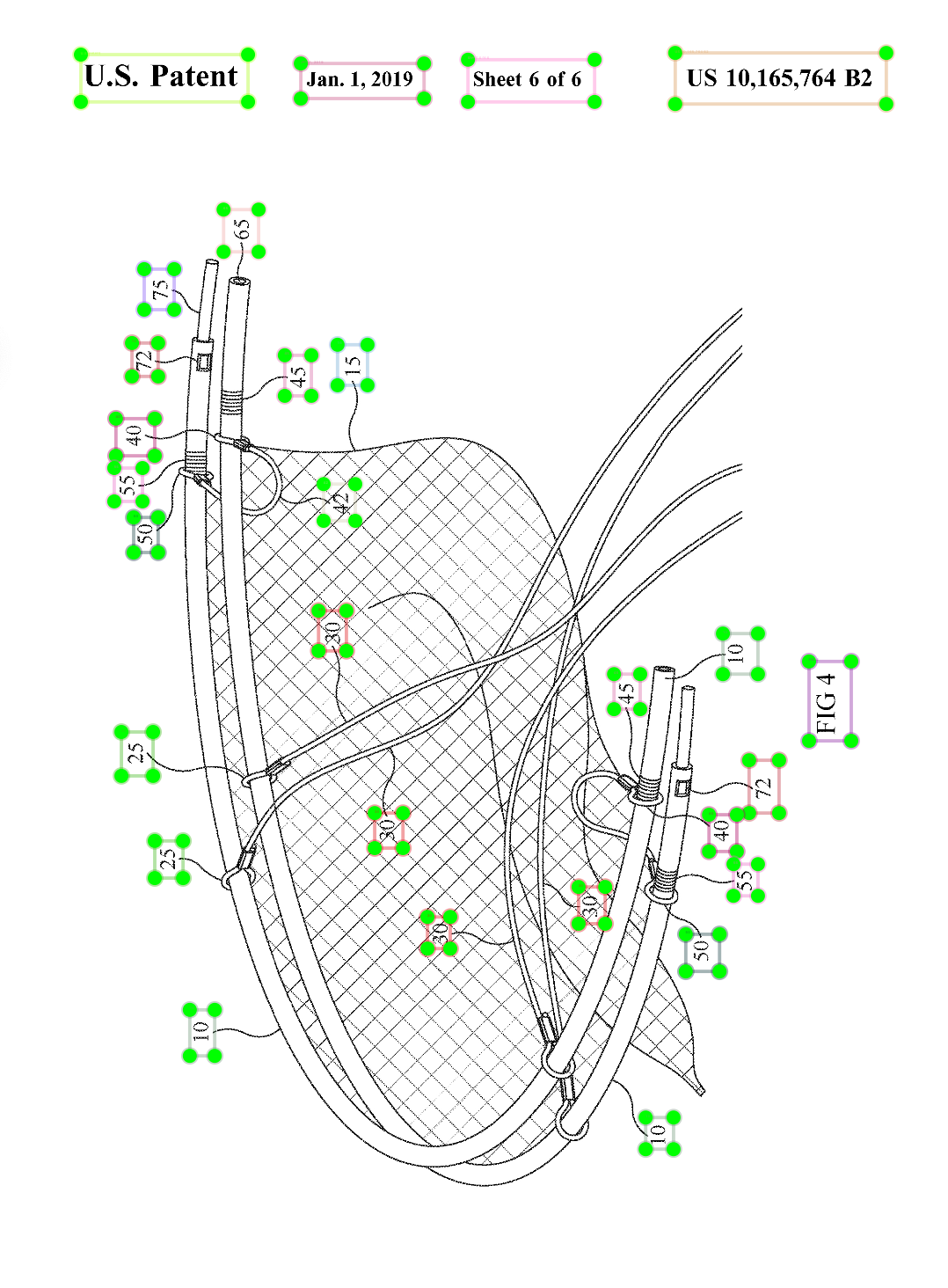
Let’s get a little bit more granular. Below is an image annotation that annotates the patents figure labels, i.e part numbers and letters.
This part of the project was something that started to become really time consuming. Each patent image has anywhere from 5 - 50 annotations. The consistency of the patent labeling isn’t 100% consistent, i.e. some patents may use a simple A., B., C., while other may use AB1, AB2, AB3. Because of this the number of patents needed to be annotated is a lot higher. From what I understand, the general heuristic is that for each given unique character there should be around 100 annotations for that same character. This heuristic is based off of OpenCV examples using character recognition on images like street signs and home addresses. Given that the format for patent text is mostly all the same, with differing fonts depending on how old the patents are, as long as the patents are within the past 10 or so years the number of annotations should probably be less than half for each character. That means for each character, the model should be able to work with 25-50 annotations – this a total guess.
One level of complexity that this adds, is that each image has to be organized into its own folder. This creates an extra layer of could needed to sort through each file recursively. Once the images are sorted by patent image itself, we can perform object detection/recognition on the labels.
Moving on
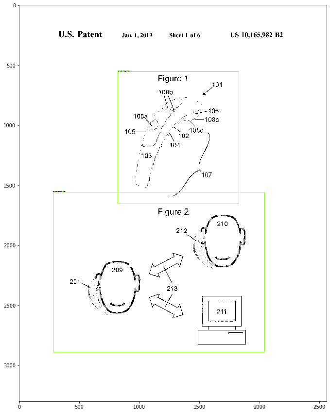
At this point in the project I decided to just keep it simple and only conduct object detection on the patent image as a whole instead of for all patent labels.
NOTE: For future reference, I think that the next alternative approach will be to look at pre-trained character recognition models.
Example multi-annotation XML file:
<annotation>
    <folder>train</folder>
    <filename>1073.jpg</filename>
    <path>/Users/home/Documents/machine_learning/models-master/space/images/train/1073.jpg</path>
    <size>
        <width>2560</width>
        <height>3300</height>
        <depth>1</depth>
    </size>
    <segmented>0</segmented>
    <object>
        <name>65</name>
        <pose>Unspecified</pose>
        <truncated>0</truncated>
        <difficult>0</difficult>
        <bndbox>
            <xmin>659</xmin>
            <ymin>560</ymin>
            <xmax>742</xmax>
            <ymax>660</ymax>
        </bndbox>
    </object>
    <object>
        <name>75</name>
        <pose>Unspecified</pose>
        <truncated>0</truncated>
        <difficult>0</difficult>
        <bndbox>
            <xmin>471</xmin>
            <ymin>701</ymin>
            <xmax>542</xmax>
            <ymax>797</ymax>
        </bndbox>
    </object>
    #
    # Repeat for each patent label figure.
    #
</annotation>
Once we have the XML files we can pull that info and place it into a single organized csv file.
The code below will recursively iterate through folders and pull the file name along with the XML info for each bounding box.
# Credit goes to 'Copyright (c) 2017 Dat Tran' https://github.com/datitran/raccoon_dataset/blob/master/xml_to_csv.py.
import os
import glob
import pandas as pd
import argparse
import xml.etree.ElementTree as ET
def xml_to_csv(path):
    xml_list = []
    for xml_file in glob.glob(path + '/*.xml'):
        tree = ET.parse(xml_file)
        root = tree.getroot()
        for member in root.findall('object'):
            value = ( root.find('filename').text, int(root.find('size')[0].text),
                      int(root.find('size')[1].text), member[0].text,
                      int(member[4][0].text), int(member[4][1].text),
                      int(member[4][2].text), int(member[4][3].text) )
            xml_list.append(value)
    column_name = ['filename', 'width', 'height', 'class', 'xmin', 'ymin', 'xmax', 'ymax']
    xml_df = pd.DataFrame(xml_list, columns=column_name)
    return xml_df
def main():
    parser = argparse.ArgumentParser(description="XML-to-CSV")
    parser.add_argument("-i", "--inputDir", help="Path to xml folder", type=str)
    parser.add_argument("-o", "--outputFile", help="Output path to csv folder", type=str)
    args = parser.parse_args()
    if(args.inputDir is None):
        args.inputDir = os.getcwd()
    if(args.outputFile is None):
        args.outputFile = args.inputDir + "/labels.csv"
    assert(os.path.isdir(args.inputDir))
    xml_df = xml_to_csv(args.inputDir)
    xml_df.to_csv(args.outputFile, index=None)
    print('Converted xml to csv.')
if __name__ == '__main__':
    main()
Example CSV file output:
| filename | width | height | class | xmin | ymin | xmax | ymax |
|---|---|---|---|---|---|---|---|
| 00000010.tif | 2560 | 3300 | 56 | 625 | 1595 | 711 | 1658 |
| 00000010.tif | 2560 | 3300 | 8 | 1213 | 465 | 1299 | 528 |
| 00000010.tif | 2560 | 3300 | 6 | 1784 | 464 | 1870 | 527 |
| 00000010.tif | 2560 | 3300 | 30 | 1246 | 893 | 1332 | 956 |
Protobuf
Next create a .pbtxt file. Pbtxt introduces the idea of protocol buffers. Protocol buffers(protobufs) are a means of serializing data. Serialization is just saying that we are te lling the computer to store or save some kind of information. For example, Python uses a Pickle file as a means of a common serialization format. Pickle is a binary format while JSON, XML, HTM, YAML, OData, and Protobufs are human readable serialization(aka data interchange) formats. Protobufs are a more universal way to serialize data and originates from Google. For more info refer to Google Protocol Bufurs. Protobufs are saved as .pb(binary) or .pbtxt(human readable) formats. These formats allow us to interchange information for effeciently as well as store information more compactly. Lastly, our .pbtxt is a place where we can store all of our annotation labels, it’s like a master record, we’ll have each unique label listed once.
Here’s a partial example of what a .pbtxt will look like:
item {
    id: 1
    name: 'patent image'
}
item {
    id: 2
    name: 'Not a patent image'
}
# If patent labels were being used here would be a few examples:
item {
    id: 3
    name: 'Patent number 10,198,1987'
}
item {
    id: 4
    name: 'A'
}
item {
    id: 5
    name: 'AB1'
}
# For each label there will be a unique id and a given name.
Optional: If there are a lot of labels then a script can be written to transfer the csv info into a .pbtxt file format.
Below is an example script that allows us to create a .pbtxt for a training/test set. The pbtxt can also be refered to as a labelmap.
filename = 'train_labels.csv'
file = pd.read_csv(filename,header=None)
file = file[3]
end = '\n'
s = ' '
ID = 1
name = 'training.pbtxt'
for x in file[1:]:
    out = ''
    out += 'item' + s + '{' + end
    out += s*2 + 'id:' + ' ' + (str(ID)) + end
    out += s*2 + 'name:' + ' ' + '\'' + str(x) + '\'' + end
    out += '}' + end
    ID += 1
    with open(name, 'a') as f:
        f.write(out)
# Grab Testing labels
filename = 'test_labels.csv'
file = pd.read_csv(filename,header=None)
file = file[3]
end = '\n'
s = ' '
ID = ID
name = 'testing.pbtxt'
for x in file[1:]:
    out = ''
    out += 'item' + s + '{' + end
    out += s*2 + 'id:' + ' ' + (str(ID)) + end
    out += s*2 + 'name:' + ' ' + '\'' + str(x) + '\'' + end
    out += '}' + end
    ID += 1
    with open(name, 'a') as f:
        f.write(out)
Moving on
Next we convert the labelmap to a tfrecord file which is a binary format for Tensorflow.
Below, class_text_to_int() allows us to convert our text labels to integer values, which will then be converted to our tfrecord format.
Usage:
  # From tensorflow/models/
  # Create train data:
  # python generate_tfrecord.py --csv_input=data/train_labels.csv  --output_path=train.record
  # Create test data:
  # python generate_tfrecord.py --csv_input=data/test_labels.csv  --output_path=test.record
from __future__ import division
from __future__ import print_function
from __future__ import absolute_import
import os
import io
import pandas as pd
import tensorflow as tf
from PIL import Image
from object_detection.utils import dataset_util
from collections import namedtuple, OrderedDict
flags = tf.app.flags
flags.DEFINE_string('csv_input', '', 'Path to the CSV input')
flags.DEFINE_string('output_path', '', 'Path to output TFRecord')
flags.DEFINE_string('image_dir', '', 'Path to images')
FLAGS = flags.FLAGS
# --------- TO-DO replace this with labelmap ------------
def class_text_to_int(row_label):
    if row_label == 'patent image':
        return 1
    else:
        None
# -------------------------------------------------------
def split(df, group):
    data = namedtuple('data', ['filename', 'object'])
    gb = df.groupby(group)
    return [data(filename, gb.get_group(x)) for filename, x in zip(gb.groups.keys(), gb.groups)]
def create_tf_example(group, path):
    with tf.gfile.GFile(os.path.join(path, '{}'.format(group.filename)), 'rb') as fid:
        encoded_jpg = fid.read()
    encoded_jpg_io = io.BytesIO(encoded_jpg)
    image = Image.open(encoded_jpg_io)
    width, height = image.size
    filename = group.filename.encode('utf8')
    image_format = b'jpg'
    xmins = []
    xmaxs = []
    ymins = []
    ymaxs = []
    classes_text = []
    classes = []
    for index, row in group.object.iterrows():
        xmins.append(row['xmin'] / width)
        xmaxs.append(row['xmax'] / width)
        ymins.append(row['ymin'] / height)
        ymaxs.append(row['ymax'] / height)
        classes_text.append(row['class'].encode('utf8'))
        classes.append(class_text_to_int(row['class']))
    tf_example = tf.train.Example(features=tf.train.Features(feature={
        'image/height': dataset_util.int64_feature(height),
        'image/width': dataset_util.int64_feature(width),
        'image/filename': dataset_util.bytes_feature(filename),
        'image/source_id': dataset_util.bytes_feature(filename),
        'image/encoded': dataset_util.bytes_feature(encoded_jpg),
        'image/format': dataset_util.bytes_feature(image_format),
        'image/object/bbox/xmin': dataset_util.float_list_feature(xmins),
        'image/object/bbox/xmax': dataset_util.float_list_feature(xmaxs),
        'image/object/bbox/ymin': dataset_util.float_list_feature(ymins),
        'image/object/bbox/ymax': dataset_util.float_list_feature(ymaxs),
        'image/object/class/text': dataset_util.bytes_list_feature(classes_text),
        'image/object/class/label': dataset_util.int64_list_feature(classes),
    }))
    return tf_example
def main(_):
    writer = tf.python_io.TFRecordWriter(FLAGS.output_path)
    path = os.path.join(FLAGS.image_dir)
    examples = pd.read_csv(FLAGS.csv_input)
    grouped = split(examples, 'filename')
    for group in grouped:
        tf_example = create_tf_example(group, path)
        writer.write(tf_example.SerializeToString())
    writer.close()
    output_path = os.path.join(os.getcwd(), FLAGS.output_path)
    print('Successfully created the TFRecords: {}'.format(output_path))
if __name__ == '__main__':
    tf.app.run()
If there are a lot of labels then use the below script which will create the script for the if else statement in the above class_text_to_int().
It takes each unique label and increments the ‘return’ statement by one.
# generate_tfrecord
# Testing
filename = 'test_labels.csv' # Comment for training set
# filename = 'train_labels.csv' # Uncomment for training set
file = pd.read_csv(filename,header=None)
file = file[3]
end = '\n'
s = ' '
ID = 0
name = 'function_test.txt' # Comment for training set
# name = 'function_train.txt' # Uncomment for training set
for x in file[2:]:
    out = ''
    out += 'elif row_label == \'' + str(x) + '\':' + end
    out += s*4 + 'return ' + str(ID) + end
    ID += 1
    with open(name, 'a') as f:
        f.write(out)
Pretrained models
Tensorflow comes with a handful of models that are pretrained. The ssd_inception_v2 is used here because it is a model that has a good balance between speed and accuracy.
NOTE: Other models can be viewed HERE.
NOTE: Corresponding config files can be viewed HERE.
We can specify our model parameters with the config file.
Default parameters are two hidden layers, l2 regularization, Relu activation function, batch size 12, .004 learning rate, 12000 train steps, 8000 eval steps.
Below is the config file.
model {
  ssd {
    num_classes: 1 # this is the number of different labels that we came across when annotating our patent images.
    image_resizer {
      fixed_shape_resizer {
        height: 300
        width: 300
      }
    }
    feature_extractor {
      type: "ssd_inception_v2"
      depth_multiplier: 1.0
      min_depth: 16
      conv_hyperparams {
        regularizer {
          l2_regularizer {
            weight: 3.99999989895e-05
          }
        }
        initializer {
          truncated_normal_initializer {
            mean: 0.0
            stddev: 0.0299999993294
          }
        }
        activation: RELU_6
        batch_norm {
          decay: 0.999700009823
          center: true
          scale: true
          epsilon: 0.0010000000475
          train: true
        }
      }
    }
    box_coder {
      faster_rcnn_box_coder {
        y_scale: 10.0
        x_scale: 10.0
        height_scale: 5.0
        width_scale: 5.0
      }
    }
    matcher {
      argmax_matcher {
        matched_threshold: 0.5
        unmatched_threshold: 0.5
        ignore_thresholds: false
        negatives_lower_than_unmatched: true
        force_match_for_each_row: true
      }
    }
    similarity_calculator {
      iou_similarity {
      }
    }
    box_predictor {
      convolutional_box_predictor {
        conv_hyperparams {
          regularizer {
            l2_regularizer {
              weight: 3.99999989895e-05
            }
          }
          initializer {
            truncated_normal_initializer {
              mean: 0.0
              stddev: 0.0299999993294
            }
          }
          activation: RELU_6
        }
        min_depth: 0
        max_depth: 0
        num_layers_before_predictor: 0
        use_dropout: false
        dropout_keep_probability: 0.800000011921
        kernel_size: 3
        box_code_size: 4
        apply_sigmoid_to_scores: false
      }
    }
    anchor_generator {
      ssd_anchor_generator {
        num_layers: 6
        min_scale: 0.20000000298
        max_scale: 0.949999988079
        aspect_ratios: 1.0
        aspect_ratios: 2.0
        aspect_ratios: 0.5
        aspect_ratios: 3.0
        aspect_ratios: 0.333299994469
        reduce_boxes_in_lowest_layer: true
      }
    }
    post_processing {
      batch_non_max_suppression {
        score_threshold: 0.300000011921
        iou_threshold: 0.600000023842
        max_detections_per_class: 100
        max_total_detections: 100
      }
      score_converter: SIGMOID
    }
    normalize_loss_by_num_matches: true
    loss {
      localization_loss {
        weighted_smooth_l1 {
        }
      }
      classification_loss {
        weighted_sigmoid {
        }
      }
      hard_example_miner {
        num_hard_examples: 3000
        iou_threshold: 0.990000009537
        loss_type: CLASSIFICATION
        max_negatives_per_positive: 3
        min_negatives_per_image: 0
      }
      classification_weight: 1.0
      localization_weight: 1.0
    }
  }
}
train_config {
  batch_size: 12 # Good friends don't let you do batch sizes over 32.
  data_augmentation_options {
    random_horizontal_flip {
    }
  }
  data_augmentation_options {
    ssd_random_crop {
    }
  }
  optimizer {
    rms_prop_optimizer {
      learning_rate {
        exponential_decay_learning_rate {
          initial_learning_rate: 0.00400000018999
          decay_steps: 800720
          decay_factor: 0.949999988079
        }
      }
      momentum_optimizer_value: 0.899999976158
      decay: 0.899999976158
      epsilon: 1.0
    }
  }
  fine_tune_checkpoint: "ssd_inception_v2_coco_2018_01_28/model.ckpt"
  from_detection_checkpoint: true
  num_steps: 12000
}
train_input_reader {
  label_map_path: 'data/object-detection.pbtxt'
  tf_record_input_reader {
    input_path: 'data/train.record'
  }
}
eval_config {
  num_examples: 8000
  max_evals: 10
  use_moving_averages: false
}
eval_input_reader {
  label_map_path: 'data/object-detection.pbtxt'
  shuffle: false
  num_readers: 1
  tf_record_input_reader {
    input_path: 'data/test.record'
  }
}
Training the model
Once we have all of the above code we can run a few commands to train our model.
Xml to csv – run for both train and test sets.
# - Create xml to csv train data:
! /Users/home/Documents/Tensorflow/scripts/preprocessing/xml_to_csv.py \
-i /Users/home/Documents/Tensorflow/workspace/training_demo/images/train \ # /test
-o /Users/home/Documents/Tensorflow/workspace/training_demo/annotations/train_labels.csv #test_labels.csv
Create TFRecord for both train and test sets.
# - Create record train data:
! \
/Users/home/Documents/Tensorflow/scripts/preprocessing/generate_tfrecord.py \
--label=patent \
--csv_input=/Users/home/Documents/Tensorflow/workspace/training_demo/annotations/train_labels.csv\ # test_labels.csv
--img_path=/Users/home/Documents/Tensorflow/workspace/training_demo/images/train \ # test
--output_path=/Users/home/Documents/Tensorflow/workspace/training_demo/annotations/train.record # test.record
Below is example output for a training model. It shows an approximate loss of 2. Ideally we want a loss of around 1
INFO:tensorflow:global_step/sec: 0.0188623
INFO:tensorflow:Recording summary at step 2749.
INFO:tensorflow:global step 2750: loss = 2.0793 (20.090 sec/step)
INFO:tensorflow:global step 2752: loss = 1.7650 (13.071 sec/step)
Once we run our model an event file will be created. This is where we can evaluate our model on Tensorboard.
# - Tensorboard Allows us to see different aspects of our data such loss, convergance, and steps taken.
!tensorboard --logdir='/Users/home/Documents/machine_learning/models-master/models/research/object_detection/training'
Now we can test our model.
# Needed libraries --
import os
import sys
import tarfile
import zipfile
import numpy as np
import tensorflow as tf
import six.moves.urllib as urllib
from object_detection.utils import ops as utils_ops
from utils import visualization_utils as vis_util # Object detection module import
from distutils.version import StrictVersion
from matplotlib import pyplot as plt
from collections import defaultdict
from utils import label_map_util # Object detection module import
from io import StringIO
from PIL import Image
%matplotlib inline
Load model, labelmap, and convert images to numpy array.
Set paths for labels and model location.
MODEL_NAME = '/Users/home/Documents/machine_learning/models-master/models/research/object_detection/patent_image_inference_graph'
PATH_TO_FROZEN_GRAPH = MODEL_NAME + '/frozen_inference_graph.pb' # Path to frozen detection graph. This is the actual model that is used for the object detection.
PATH_TO_LABELS = os.path.join('/Users/home/Documents/machine_learning/models-master/models/research/object_detection/data/', 'object-detection.pbtxt') # Adds label for each box.
# Load Tensorflow model:
detection_graph = tf.Graph()
with detection_graph.as_default():
    od_graph_def = tf.GraphDef()
    with tf.gfile.GFile(PATH_TO_FROZEN_GRAPH, 'rb') as fid:
    serialized_graph = fid.read()
    od_graph_def.ParseFromString(serialized_graph)
    tf.import_graph_def(od_graph_def, name='')
# Load label map:
category_index = label_map_util.create_category_index_from_labelmap(PATH_TO_LABELS, use_display_name=True)
# Loads image into usable format, numpy array.
def load_image_into_numpy_array(image):
    # Function supports only grayscale images
    last_axis = -1
    dim_to_repeat = 2
    repeats = 3
    grscale_img_3dims = np.expand_dims(image, last_axis)
    training_image = np.repeat(grscale_img_3dims, repeats, dim_to_repeat).astype('uint8')
    assert len(training_image.shape) == 3
    assert training_image.shape[-1] == 3
    return training_image
Create test function.
PATH_TO_TEST_IMAGES_DIR = '/Users/home/Documents/machine_learning/models-master/models/research/object_detection/test_images'
TEST_IMAGE_PATHS = [ os.path.join(PATH_TO_TEST_IMAGES_DIR, 'image{}.jpg'.format(i)) for i in range(3, 12) ]
IMAGE_SIZE = (25, 20)
def run_inference_for_single_image(image, graph):
    with graph.as_default():
        with tf.Session() as sess:
            # Get handles to input and output tensors
            ops = tf.get_default_graph().get_operations()
            all_tensor_names = {output.name for op in ops for output in op.outputs}
            tensor_dict = {}
            for key in ['num_detections', 'detection_boxes', 'detection_scores', 'detection_classes', 'detection_masks']:
                tensor_name = key + ':0'
                if tensor_name in all_tensor_names:
                    tensor_dict[key] = tf.get_default_graph().get_tensor_by_name(tensor_name)
            if 'detection_masks' in tensor_dict:
                # The following processing is only for a single image
                detection_boxes = tf.squeeze(tensor_dict['detection_boxes'], [0])
                detection_masks = tf.squeeze(tensor_dict['detection_masks'], [0])
                # Reframe is required to translate mask from box coordinates to image coordinates and fit the image size.
                real_num_detection = tf.cast(tensor_dict['num_detections'][0], tf.int32)
                detection_boxes = tf.slice(detection_boxes, [0, 0], [real_num_detection, -1])
                detection_masks = tf.slice(detection_masks, [0, 0, 0], [real_num_detection, -1, -1])
                detection_masks_reframed = utils_ops.reframe_box_masks_to_image_masks(detection_masks, detection_boxes, image.shape[1], image.shape[2])
                detection_masks_reframed = tf.cast(
                    tf.greater(detection_masks_reframed, 0.5), tf.uint8)
                # Follow the convention by adding back the batch dimension
                tensor_dict['detection_masks'] = tf.expand_dims(detection_masks_reframed, 0)
            image_tensor = tf.get_default_graph().get_tensor_by_name('image_tensor:0')
            # Run inference
            output_dict = sess.run(tensor_dict, feed_dict={image_tensor: image})
            # all outputs are float32 numpy arrays; convert types as needed
            output_dict['num_detections'] = int(output_dict['num_detections'][0])
            output_dict['detection_classes'] = output_dict['detection_classes'][0].astype(np.int64)
            output_dict['detection_boxes'] = output_dict['detection_boxes'][0]
            output_dict['detection_scores'] = output_dict['detection_scores'][0]
            if 'detection_masks' in output_dict:
                output_dict['detection_masks'] = output_dict['detection_masks'][0]
    return output_dict
Run test and view image results.
for image_path in TEST_IMAGE_PATHS:
    image = Image.open(image_path)
    # Array representation of image will be used later to prepare result image w/ boxes &* labels.
    image_np = load_image_into_numpy_array(image)
    image_np_expanded = np.expand_dims(image_np, axis=0)
    output_dict = run_inference_for_single_image(image_np_expanded, detection_graph)     # Actual detection.
    # Visualization of the results of a detection.
    vis_util.visualize_boxes_and_labels_on_image_array(image_np,
                                                       output_dict['detection_boxes'],
                                                       output_dict['detection_classes'],
                                                       output_dict['detection_scores'],
                                                       category_index,
                                                       instance_masks=output_dict.get('detection_masks'),
                                                       use_normalized_coordinates=True,
                                                       line_thickness=4)
    plt.figure(figsize=IMAGE_SIZE)
    plt.imshow(image_np)
Results
The results were upper 90s for accuracy.
NOTE: remember to add other random images to your test set, this can be both random images and text images from the patent data.
Next steps:
- Train new object detection model to detect image figure numbers; use a pretrained character recognition model.
- Parse patent text data to tokenize and formalize patent image data and image figures data.